Example FAIR analysis
This is an example of a risk analysis using the FAIR model implemented in an R Markdown Notebook. When you execute code within the notebook, the results appear beneath the code.
Estimates from Subject Matter Experts
Estimates should be calibrated. There are good courses available on calibrating your subject matter experts.
Estimates are all provided as a range of min, max, and most likely. For advanced analysis, you can also tweak the confidence factor to adjust the shape of the distribution.
Set up inputs for Loss Event Frequency
If loss event freqency cannot be estimated, then go a level deeper in the FAIR model and derive loss event frequency from Threat Event Frequency and Vulnerability (susceptibility). For the purpose of this example we will estimate Loss Event Frequency directly.
We are estimating that this loss occurs at least twice a year, is most likely to happen 4 times a year (once per quarter), and at most would occur 9 times per year.
loss_event_frequency_min <- 2
loss_event_frequency_max <- 9
loss_event_frequency_likely <- 4
Set up inputs for Loss Magnitude
Losses in FAIR are divided into primary losses and secondary losses. Another term for this is guaranteed losses and conditional losses. Primary losses are typically where we put losses incurred directly by the organization, Secondary losses are typically where we put losses that are caused by actions that secondary stakeholders might take. If a secondary loss always occurs, there is no math reason for categorizing as a secondary loss.
Losses in FAIR are divided into 6 forms, to help structure the discussion with your subject matter experts. All the forms of loss get added together, but dividing them in this way helps organize the calculations.
The 6 forms of loss in FAIR are
- Productivity Loss - lost sales, idle employees
- Response costs - hiring lawyers, forensic investigations, generators
- Replacement costs
- Competitive Advantage
- Fines/Judgements
- Reputation Damage - examples are uncaptured revenue, increased cost of capital
In this example we will not calculate each form of loss separately, but assume that we have considered each of those forms and come up with a range estimate of loss magnitude.
loss_magnitude_min <- 1000
loss_magnitude_max <- 9000
loss_magnitude_likely <- 4000
Run the calculations
confidence <- 4 # default in PERT
number_of_runs <- 10000
We do a monte carlo simulation using the beta-PERT distribution. Defaulting to 10,000 runs. Confidence level of 4 is the default in beta-PERT, we can vary this value to change the shape of the distribution to reflect lower or higher certainty around the most likely value.
For a nice explanation of how this code works in R, see this explanation of betaPERT by Jay Jacobs
Set a seed for repeatable results in this notebook
set.seed(88881111)
Run the simulation for the Loss Event Frequency
LEF <- rpert(number_of_runs, loss_event_frequency_min, loss_event_frequency_likely, loss_event_frequency_max, shape = confidence)
Run the simulation for the Loss Magnitude
LM <- rpert(number_of_runs, loss_magnitude_min, loss_magnitude_likely, loss_magnitude_max, shape = confidence)
Multiply Loss Event Frequency x Loss Magnitude. Note that in R this is doing vector multiplication.
annual_loss_exposure <- LEF * LM
crude_ALE <- annual_loss_exposure
Simple vector multiplication as implied by the FAIR model assumes that multiple losses in a single year are the same size, for a better approach described at Severski we can take each set of loss events in a year and sample from the distribution of loss magnitudes, then sum.
ALE <- sapply(LEF, function(e) sum(rpert(e, loss_magnitude_min, loss_magnitude_likely, loss_magnitude_max, shape = confidence)))
max_loss <- max(ALE)
min_loss <- min(ALE)
Take the 95th percentile for the first result. Value at Risk is $40,123.11. Maximum Loss is $60,447.74. Mean Loss is $19,499.58. Minimum Loss is $3,029.60.
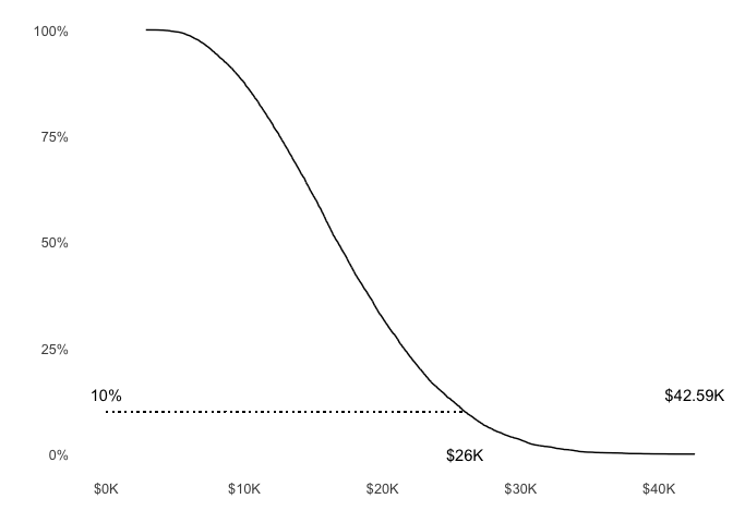
Take the 95th percentile. Value at Risk is $30,648.46. Maximum Loss is $42,587.60. Mean Loss is $17,292.94. Minimum Loss is $2,864.44.
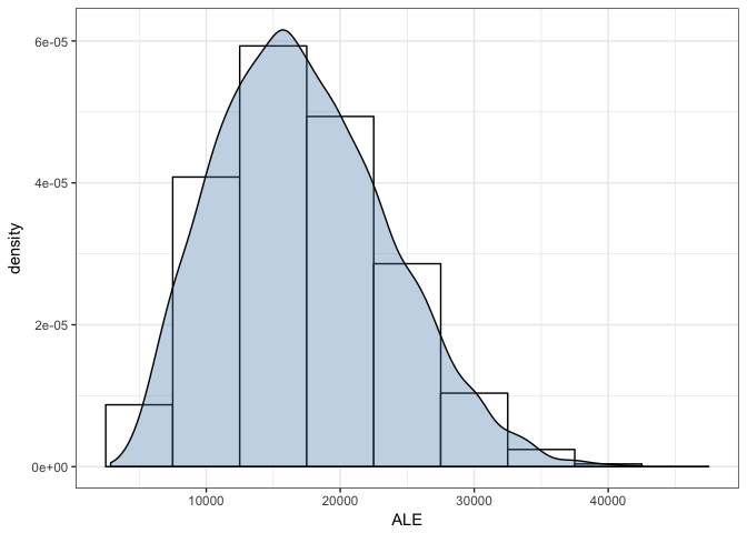
Histogram visualization
Plot the results to show annual loss exposure. This can be plotted as a histogram or a loss exceedance curve with linear or exponential scales.
ale_frame <- data.frame(ALE)
most <- max(ALE)

gg <- ggplot(ale_frame, aes(x = ALE))
gg <- gg + geom_histogram(aes(y = ..density..),
                          color="black",
                          fill = "white",
                          binwidth = 5000)
gg <- gg + geom_density(fill = "steelblue", alpha = 1/3)
gg <- gg + theme_bw()
gg
Loss Exceedance curve
Lets look at the loss exceedance curve for these results.
# calculate the probability of exceedance aka complementary cumulative probability function
ale_frame <- mutate(ale_frame, prob = 1 - percent_rank(ALE))
# sort the results in ascending order of loss magnitude
ale_frame <- ale_frame[order(ALE),]
g2 <- ggplot(ale_frame, mapping = aes(x = ALE, y = prob))
g2 <- g2 + geom_path() + scale_y_continuous(labels = percent)
#g2 <- g2 + geom_hline(yintercept = 0.1, color = "red", size = .5) +
#  scale_y_continuous(labels = percent)

g2 <- g2 + scale_x_continuous(labels = format_kdollars) # normal scale
#g2 <- g2 + scale_x_log10(labels = format_kdollars) # logarithmic scale
g2 <- g2 + annotate("text", y = 0.1, x = max(ALE),
                    label = format_kdollars(max(ALE)), vjust = -1)
#g2 <- g2 + geom_hline(yintercept = 0.1, lty = "dotted")
#g2 <- g2 + geom_vline(xintercept = max(ale_frame$ALE), lty = "dotted")
g2 <- g2 + annotate("text", y = 0.10, x = 0, label = percent(0.1), vjust = -1)
g2 <- g2 + annotate("text", y = 0, x = quantile(ale_frame$ALE, c(0.90)),
                    label = format_kdollars(round(quantile(ale_frame$ALE, c(0.90)), digits = -2)), hjust = 0.5)

g2 <- g2 + geom_segment(aes(x = 0, y = 0.1, xend = quantile(ale_frame$ALE, c(0.90)), yend = 0.1), lty = "dotted")
#           geom_point(data = intersection_xy_df, size = 3)
g2 + theme_few()
Notes
It’s important to note that this is not a prediction, but a calculation of probabilities. Even if something is only 1% probable, it could still happen. It’s also important to note all the assumptions made in the risk scenario being analyzed and in the estimates used as inputs to the model.